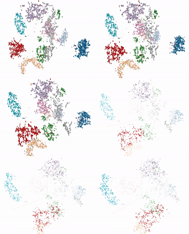
t-SNE is a state of the art algorithm for dimentionality reduction. This algorithm is used for mainly pre-processing of machine learning. You may know PCA as similar algorithm. Though both techniques are useful for capturing the specific feature of the data set space, t-SNE is more powerful even with huge dimensional datasets.
In this post, I want to explain a overview of t-SNE and introduce a tool I made in order to try t-SNE easily on your data sets.
t-SNE
t-SNE is an abbreviation of t-distributed stochastic neighbor embedding. What t stands for? t-SNE uses student-t distribution internally. So it’s named after that distribution. t-SNE expresses the similarity of each points by using probabilistic distribution. Assuming we want to calculate the similarity between a point \(x_i\) and others. We can define the distance from the point \(x_i\) to \(x_j\) as \(P_{j|i}\). The nearer \(x_j\) is from \(x_i\), the smaller the distance is. The distance can be defined as probability.
\begin{equation} P_{j|i} = \frac{exp(-|x_i - x_j|^2/2 \sigma_i^2)}{\sum_{k \neq i} exp(-|x_i - x_k|^2 / 2\sigma_i^2)}, P_{i|i} = 0 \end{equation}
\begin{equation} P_{i, j} = \frac{P_{j|i} + P_{i|j}}{2N} \end{equation}
\(P_{j\|i}\) is a conditional probability. \(P_{i, j}\) is simultaneous probability of each points. This is the similarities of each point in original data space. Then we can calculate the similarities in projected space after dimentionality reduction. We assume it \(Q_{j,i}\). The points of this is we calculate the \(Q\) by using student’s t-distribution. In short
\begin{equation} Q_{i|j} = \frac{(1+|y_i - y_j|^2)^{-1}}{\sum_{k \neq i} (1+|y_i - y_k|^2)^{-1}}, Q_{i|i} = 0 \end{equation}
\(y_i\) is a projected point from \(x_i\) in original space. So what we want to do is making \(Q_{i,j}\) and \(P_{i,j}\) similar. The similarity between two probabilistic distribution can be calculated by KL divergence. KL divergence between \(P_{i,j}\) and \(Q_{i,j}\) is this.
\begin{equation} C = \sum_{i} \sum_{j} P_{i,j} log \frac{P_{i,j}}{Q_{i,j}} \end{equation}
Optimization of cost function \(C\) should provide the best distribution \(Q_{i,j}\) with corresponding data sets \(y_i\). The optimization is calculated stochastic gradient descent as the algorithm name suggested.
tf-sne
So let’s take a look of the MNIST data points after t-SNE. MNIST is a famous hand written digit data set. We use this data sets as example of t-SNE projection. tf-sne is a light tool weight visualization tool using Tensorflow. Tensorflow provides a tool to investigate the loss function value or embedded data point space, called Tensorboard. So what tf-sne does is
- Convert given data set into the Tensorflow model format to be read Tensorboard
- Launch Tensorboard which provides PCA and t-SNE projector to visualize data points
tf-sne can read the data point in csv format like this. And you might want to add labels to each point. Please provide it as metadata_file in csv format. One thing to note is features_file and metadata_file must contain same number of data points in same order. Otherwise wrong label can be attached in visualization dashboard. Please check metadata detail if necessary.
$ docker run -it \
  -p 6006:6006 \
  -v ${DATA_DIR}:/srv/tf-sne/data \ # Specify the directory contains input data
  lewuathe/tf-sne  \
  --features_file features.csv \
  --metadata_file metadata.csv
Then you can see interactive t-SNE dashboard in http://localhost:6006.

Thanks!